R语言学习：R4DS学习、6种join操作理解、case_when函数理解、ggplot2包做数据可视化

2022-8-21 萌小白

2021年第39周。

这一周R语言学习，记录如下。

Modern Statistics with R

一本在线开放书籍，介绍R语言做数据整理和探索，以及推断和预测的工作。

访问网址：

http://www.modernstatisticswithr.com/

R4DS书籍

最近，我在重温R4DS这本书籍。

你所想的数据科学是什么？

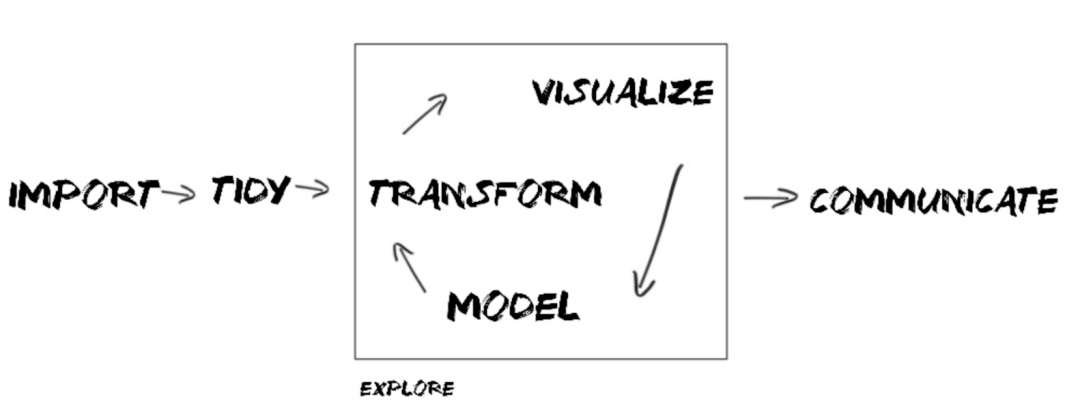
实际中的数据科学是什么？

数据的准备工作，需要花费大部分时间。

我创建了R4DS学习群，加我的微信，备注：R4DS，邀请你入群，大家一起学习，同时，也会分享R4DS相关的资料。

dplyr包的join系列函数

数据关联是数据集成和整合的常用操作。

dplyr包提供了一组功能强大的join函数集，可以方便地实现数据的关联。

1 inner_join函数

2 left_join函数

3 right_join函数

4 full_join函数

5 semi_join函数

6 anti_join函数

关于这6种join操作，你理解了吗?有任何问题或者想法，请加入R4DS学习群，一起讨论。

样本选择

dplyr包的filter函数提供了强大的样本选择功能。

filter函数理解。

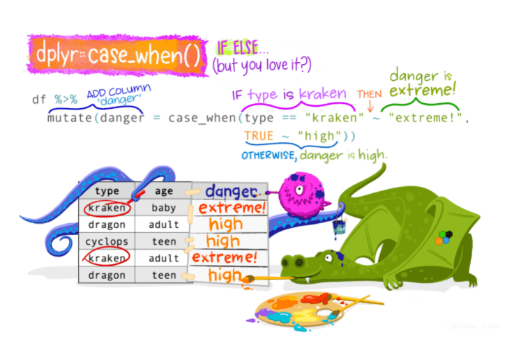
case_when函数理解

dplyr包的case_when函数实现开关选择操作。

case_when函数理解。

R4DS第一章 ggplot2包与数据可视化简要笔记

1 为什么需要数据可视化？

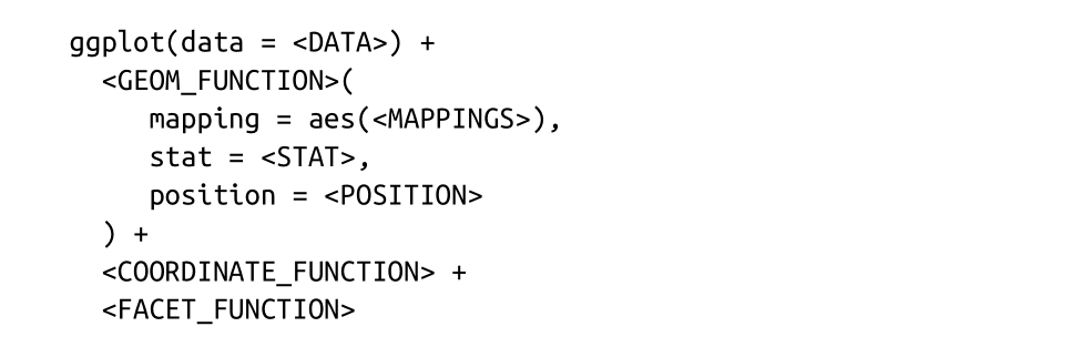
2 ggplot2包做数据可视化的逻辑

图形语法+分层架构

3 内容结构

1）准备工作

2）以研究mpg数据displ与hwy的关系的问题做引子，介绍利用数据可视化技术做图形化分析

3）接下来介绍ggplot画图的重要组件

Aesthetic Mapping

Facets

Geometric Objects

Statistical Transformations

Position Adjustments

Coordinate Systems

4) 图形学的分层语法

4 目标管理

1）理解ggplot2包画图的基本逻辑和原理。

2）掌握常用的5种图形，散点图、条形图、盒箱图、直方图、点线图。

3）学会用图形化思维对数据做探索、理解和表达。

5 实操代码

graphics.off()

rm(list = ls())

options(warn = -1)

options(scipen = 999)

options(digits = 3)

# R4DS第一章 ggplot2包与数据可视化

# 准备工作

library(tidyverse)

# 数据可视化的流程

# 提问题--找数据--选图形--做图形--得信息--导行动

# 例如：想了解引擎尺寸和燃油效率的关系？

# 正向还是负向；线性还是非线性？

# 使用自带的mpg数据库

data(mpg)

mpg %>% glimpse()

mpg %>% head

help(mpg)

# 找到数据集，需要寻找或者构建与问题相关的变量或者特征

# 1）displ 引擎的尺寸

# 2）hwy 燃油效率每加仑油对应的行驶距离相同距离下，高效率相对于低效率需要更少的油

# 绘制图形

# 探索两个变量之间的关系

# 变量数目： 2个

# 变量类型：连续型

# 采用散点图

# 根据变量的类型和数目，选择合适的图形

# 坐标轴 x--displ y--hwy

ggplot( data= mpg) +

geom_point(aes(x = displ, y = hwy))

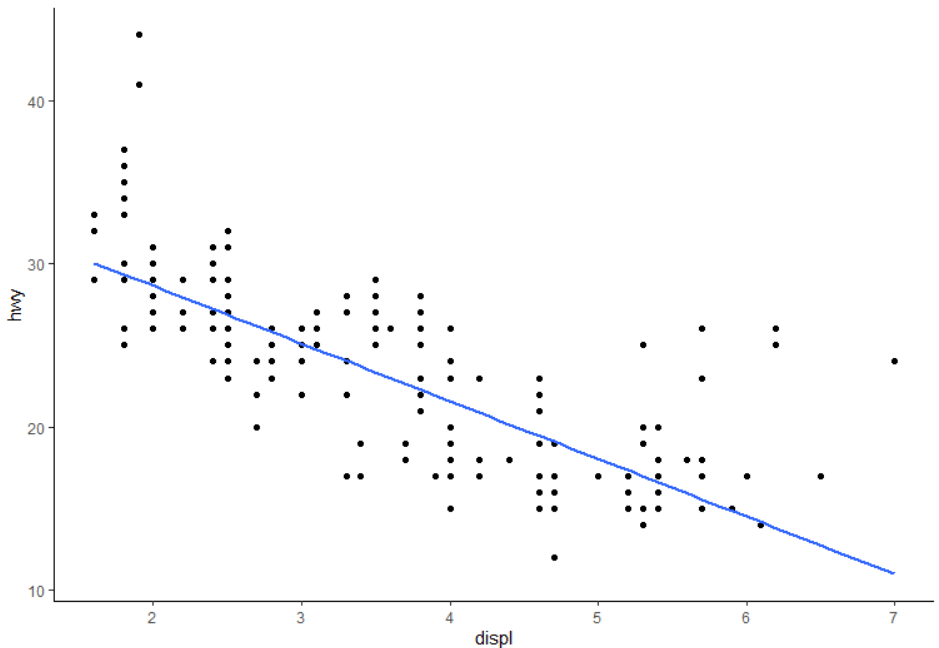
ggplot( data= mpg, aes(x = displ, y = hwy)) +

geom_point() +

geom_smooth(method = 'lm', se = FALSE)

ggplot( data= mpg, aes(x = displ, y = hwy)) +

geom_point() +

geom_smooth(method = 'lm', se = FALSE) +

theme_classic()

# 必要三组件

# 1）数据集

# 2）几何图形对象

# 3）映射关系，变量映射到坐标轴、尺寸、颜色、透明度等

# 通用模板

# ggplot( data= <DATA>) +

# <GEOM_FUNCTION>(mapping = aes(<MAPPING>))

# 练习 1

ggplot( data= mpg)

mpg %>% glimpse()

?mpg

ggplot( data= mpg) +

geom_point(aes(x = cyl, y = hwy))

ggplot( data= mpg) +

geom_point(aes(x = drv, y = class))

# 思考：

# 一幅简洁的图能够带来什么信息？

# 差异化标识

ggplot( data= mpg) +

geom_point(aes(x = displ, y = hwy, color = class))

# 分面板观察

ggplot( data= mpg) +

geom_point(mapping = aes(x = displ, y = hwy)) +

facet_wrap(~ class, nrow = 2)

ggplot( data= mpg) +

geom_point(mapping = aes(x = displ, y = hwy)) +

facet_grid(drv ~ cyl)

ggplot( data= mpg) +

geom_point(mapping = aes(x = displ, y = hwy)) +

facet_grid(. ~ cyl)

ggplot( data= mpg) +

geom_point(mapping = aes(x = displ, y = hwy)) +

facet_grid(drv ~ .)

# 不同的画图几何对象

ggplot( data= mpg) +

geom_point(mapping = aes(x = displ, y = hwy))

ggplot( data= mpg) +

geom_smooth(mapping = aes(x = displ, y = hwy))

ggplot( data= mpg) +

geom_smooth(mapping = aes(x = displ, y = hwy, linetype = drv))

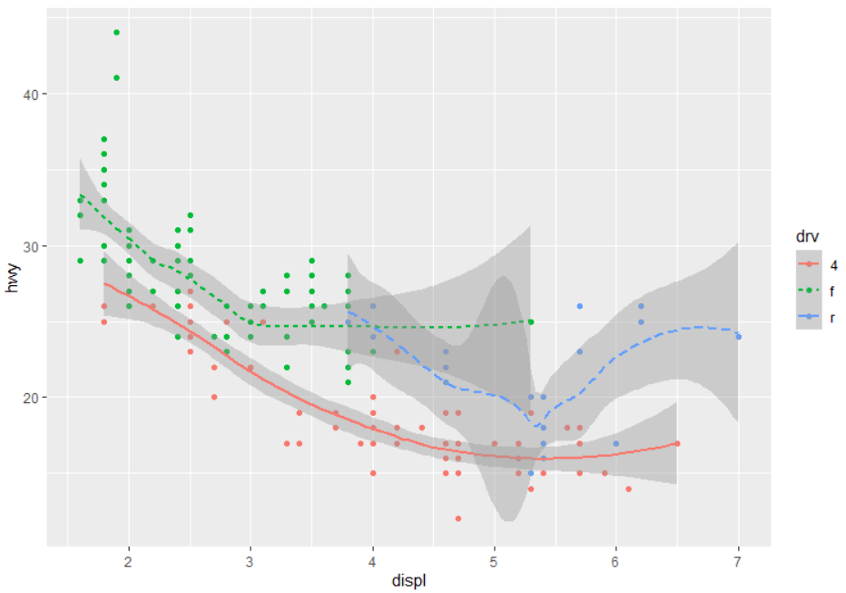
ggplot( data= mpg) +

geom_point(mapping = aes(x =displ, y = hwy, color = drv)) +

geom_smooth(mapping = aes(x = displ,

y = hwy,

linetype = drv,

color = drv))

# 添加趋势线

ggplot( data= mpg) +

geom_smooth(mapping = aes(x = displ, y = hwy))

ggplot( data= mpg) +

geom_smooth(mapping = aes(x = displ,

y = hwy,

group = drv))

ggplot( data= mpg) +

geom_smooth(mapping = aes(x = displ,

y = hwy,

color = drv),

show.legend = FALSE)

ggplot( data= mpg) +

geom_point(mapping = aes(x = displ, y = hwy)) +

geom_smooth(mapping = aes(x = displ, y = hwy))

ggplot( data= mpg, mapping = aes(x = displ, y = hwy)) +

geom_point() +

geom_smooth()

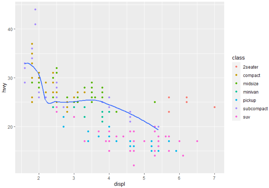
ggplot( data= mpg, mapping = aes(x = displ, y = hwy)) +

geom_point(mapping = aes(color = class)) +

geom_smooth()

ggplot( data= mpg, mapping = aes(x = displ, y = hwy)) +

geom_point(mapping = aes(color = class)) +

geom_smooth(

data= filter(mpg, class== "subcompact"),

se = FALSE

)

# 统计变换

ggplot( data= diamonds) +

geom_bar(mapping = aes(x = cut))

ggplot( data= diamonds) +

stat_count(mapping = aes(x = cut))

# 参数stat明示化的 3种情况

# 构造数据集

demo <- tribble(

~a, ~b,

"bar_1", 20,

"bar_2", 30,

"bar_3", 40

)

ggplot( data= demo) +

geom_bar(

mapping = aes(x = a, y = b),

stat= 'identity'

)

# 绘制每一组的百分比

ggplot( data= diamonds) +

geom_bar(

mapping = aes(x = cut, y = ..prop.., group = 1)

)

# 统计图形可视化

ggplot( data= diamonds) +

stat_summary(

mapping = aes(x = cut, y = depth),

fun.min = min,

fun.max = max,

fun= median

)

# 位置调整

ggplot( data= diamonds) +

geom_bar(mapping = aes(x = cut, color = cut))

ggplot( data= diamonds) +

geom_bar(mapping = aes(x = cut, fill = cut))

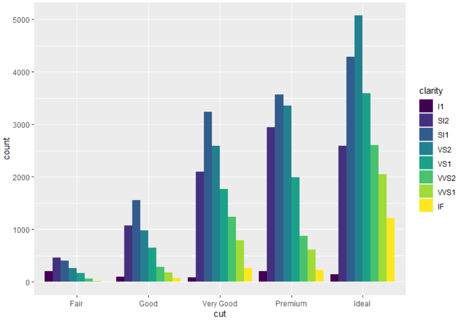
ggplot( data= diamonds) +

geom_bar(mapping = aes(x = cut, fill = clarity))

ggplot(

data= diamonds,

mapping = aes(x = cut, fill = clarity)

) +

geom_bar(alpha = 1/ 5, position = 'identity')

ggplot(

data= diamonds,

mapping = aes(x = cut, color = clarity)

) +

geom_bar(fill = NA, position = 'identity')

ggplot(

data= diamonds

) +

geom_bar(

mapping = aes(x = cut, fill = clarity),

position = 'fill'

)

ggplot(

data= diamonds

) + geom_bar(

mapping = aes(x = cut, fill = clarity),

position = "dodge"

)

ggplot(

data= mpg

) + geom_point(

mapping = aes(x = displ, y = hwy),

position = "jitter"

)

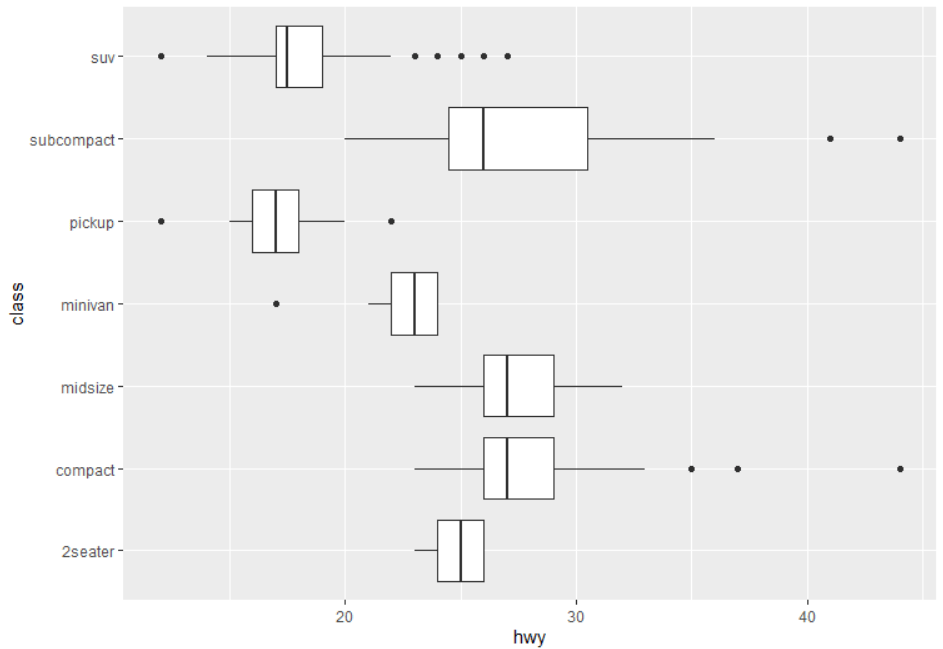
# 坐标系统

ggplot( data= mpg, mapping = aes(x = class, y = hwy)) +

geom_boxplot()

ggplot( data= mpg, mapping = aes(x = class, y = hwy)) +

geom_boxplot() +

coord_flip()

nz <- map_data( "nz")

ggplot(nz, aes(long, lat, group = group)) +

geom_polygon(fill = "white", color = "black")

ggplot(nz, aes(long, lat, group = group)) +

geom_polygon(fill = "white", color = "black") +

coord_quickmap()

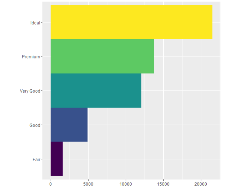
bar <- ggplot( data= diamonds) +

geom_bar(

mapping = aes(x = cut, fill = cut),

show.legend = FALSE,

width = 1

) +

theme(aspect.ratio = 1) +

labs(x = NULL, y = NULL)

bar + coord_flip()

bar + coord_polar()

6 部分结果展示（大家可以自测代码）

可重复性代码构建指南

创建项目工程，做项目管理

项目的层级架构，参考下图：

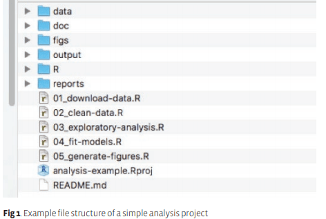
各个文件夹和文件的用途

请注意

1 永远不要修改原始数据，或者说，一定要备份好原始数据

2 对于任何项目，创建一个文件，记录你的所思和所做，便于复盘和迭代

3 脚本的命名，请知名晓意，赋予含义，具有条理性和逻辑性，重视代码的可读性，代码是让电脑来运行的，更重要的是，让人来看的。

4 对于一个复杂的项目，编写代码之前，先写伪代码或者画流程图

md5加密

实际工作中，有时候需要抽取内部数据与第三方数据做撞库操作。这个时候，需要把敏感信息，比方说，身份证号码、手机号码、姓名做加密处理，常用md5加密。

digest包的digest函数，可以方便地进行md5加密。

library(diges)

id1 <- "1234567890"

id1

id1_md5 <- digest(id1, algo = "md5", serialize = FALSE)

id1_md5

补充信息

源自：https://github.com/BaHui/MD5Hash

MD5加密是最常用的不可逆加密方法之一，是将字符串通过相应特征生成一段32位的数字字母混合码。对输入信息生成唯一的128位散列值（32个16进制的数字)

但是常见的会有16位和32位长度之分, 实际上MD5产生的就是唯一的32位的长度, 所谓的16位的长度可以理解为对MD5的再加工而形成的. 再加工就是: 32 位字符串中，取中间的第 9 位到第 24 位的部分

dplyr包across函数

dplyr包across函数，把一个函数或者一系列函数应用到一些具有某种模式下的列做处理。

# dplyr包across函数

library(dplyr)

library(magrittr)

help( package= 'dplyr')

iris %>%

group_by(Species) %>%

summarise(across(starts_with( "Sepal"), mean), .groups = "drop") %>%

View

iris %>%

group_by(Species) %>%

summarise(across(starts_with( "Sepal"), list(mean = mean, sd = sd)), .groups = "drop") %>%

发表评论：